Ultra Fractal Tutorial -- Solid Color -- Part One
by Robert "Red" Williams

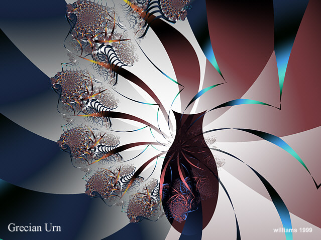
When I published a variation on Luke Plant's "Scissors" transformation, followed by the similar, but more complex, "Shapes", I discovered that the workings of the "Solid Color" feature of Ultrafractal was not well understood by many. To my surprise, this incomplete understanding extended to some of the more experienced and innovative UF users. I have since added a fourth member, "Regular Polygons", to this family of transformation routines. Together, these four routines constitute an extremely powerful tool for manipulation and control of our images. Anyone who doubts that should take a look at my composition, Symbols or at the more subtle Grecian Urn.

This explanation, along with the examples and illustrative parameter sets, is intended to familiarize you with the concept of the "Solid Color" and acquaint you with some basic techniques for exploiting its features.

People often refer to inside color and solid color as if they were synonymous and polar opposites of so-called outside color. The terms inside and outside refer to the Mandlebrot set - points in the set are traditionally colored black while the coloring of outside points is usually governed by some set of coloring rules based on the way the result changes as the formula is iterated. However, inside points may be colored according to a set of rules and outside points may be assigned a single color; after all, "color all outside points chartreuse" is a coloring rule and inside points may follow complex orbits despite the fact that they never escape.

If you click on the Inside Tab, you will see a little black Mandelbug at the right side of the dialog box. Click on it and a pop-up dialog box labeled "Solid Inside" will appear. You may use its input boxes to specify a color directly, using either the RGB or HSL model or, if you prefer, click on the checkerboard icon at the upper left and a color picker will pop up, from which you may select a color. There is also an input box labeled "Opacity" into which you may enter a number from 0 to 255. This controls the transparency of the solid color in much the same manner as the Opacity Slider on the Layers Tab controls the transparency of the entire layer. Zero means 100% transparent and 255 is opaque.

There are similar icons on the right side of the Outside Tab and the left side of the Mapping Tab. If there is no transformation loaded, the icon on the Mapping tab will be "greyed out". Clicking on these icons will produce similar pop-up dialog boxes labeled "Solid Outside" and "Solid Mapping". These are all independent, enabling you to specify three solid colors, each with its own degree of opacity.

In order to follow the rest of the discussion, you'll need to render this UPR.

This image demonstrates all three types of solid color. Layer 2 has a Scissors transform loaded and Inside, Outside, and Mapping are all assigned different solid colors. Turn Layers 3 and 4 off and select Layer 2. Then click on the alpha symbol on Layer 2. You will see a blue field with an orange Mandelbrot figure in the center and a green astroid in the upper right. These three colors are the three solid colors I chose for Outside, Inside and Mapping, respectively. Now, click on the alpha symbol again and because all three colors are partially transparent, you will see Layer 1 showing through them again. Then turn off Layer 1 and you will see the image revert to the same appearance that it had when the alpha symbol was "grayed out". This demonstrates that, if there is no underlying layer, the transparency will have no effect - you will see only the solid colors as if they were 100% opaque. This can be confusing when you're working. It is easy to turn off the underlying layers and then you can't figure out why the transform doesn't seem to be working right. So, if you ever think things aren't behaving as they should, make sure there is a visible layer under the one with transparent areas.

Layer 3 is exactly the same as Layer 2 except that the solid colors are all completely transparent. Turn off Layer 2 and make Layer 3 visible. Now, when you click on the alpha symbol, the layer is either completely opaque or completely transparent so when the symbol is greyed out, you see only the solid colors - click again and the layer is entirely invisible.

Now, as you have seen, clicking on the alpha symbol affects all solid colors together; however, they may be controlled individually, as well. The Transform can be activated or inactivated by clicking on its icon. The Inside and Outside solid colors may be activated by clicking on Transfer Function and selecting None from the drop-down menu. Selecting any other transfer function activates whatever coloring method has been selected. Note: Transfer Function = None is not the same as Coloring Method=None.

So, to summarize, you can have up to three solid color assignments, each in its own color and corresponding degree of transparency. They may be activated together by the alpha symbol on the Layers Tab or individually by Transfer Function selection or the Transform icon, as appropriate.

NOTE: The Alpha Channel is entirely independent of Solid Color designations and does not affect areas assigned the Solid Color, but if you have also created an alpha channel for the layer, it will be activated or deactivated by clicking on the alpha symbol, too. You must take this into account as you work on an image, presumably, you won't be turning effects on and off except to evaluate progress as you work.

Next, if you make Layers 2 and 3 invisible and select Layer 4, you will see a sort of racetrack-shaped area at the upper left. This is the reverse of Scissors - the area around the shape is partially transparent and the shape itself is opaque. If you deactivate the transform by clicking on the the transform icon on the Mapping Tab, you will see the entire layer. If you click on the alpha symbol, you will see the solid color which is the same ugly green you've already seen on Layers 2 and 3.

You might well wonder why there are so many transforms to do such similar things. The reason is that the interface between Ultrafractal proper and the transformation algorithms doesn't permit a pixel to be redesignated once it has been assigned the solid color. This means that you can load in multiple Scissors transforms and create a composite of several transparent shapes, but you cannot do the same thing with opaque shapes such as Reverse Scissors creates. If you load a second Reverse Scissors transform, the transparent area surrounding each shape "erases" the other shape. That's why I wrote Shapes - it allows you to define up to ten separate shapes before the final assignment of solid colored pixels is made; therefore, you can create an aggregate of several shapes. Regular Polygons does the same thing as Shapes except, as the name implies, it makes regular polygons (and a five-pointed star) instead of ellipses, etc. In Shapes and Regular Polygons, you may specify that either the area inside or outside the figure is the solid color. This means that the figure may be either transparent or opaque as you choose.

Some comments on the shapes available seem justified at this point. Regular polygons are pretty well self-explanatory - the transformation provides all of them with from 3 to 10 sides and the even-numbered from 12 to 20 sides, inclusive. It also "throws in" a five-pointed star for no other reason than that I realized I could do it. Rectangle is obvious, as is ellipse and if height and width are equal, the former becomes a square and the latter, a circle. Astroid is not so obvious but it is nothing more than a special case of the "General" shape. The General shape is so-named because it uses the general form of an equation which describes a particular family of closed figures. For those who are interested in such things, the equation is: (x/a)^n + (y/b)^n =1. At the risk of insulting someone, such equations may be solved to create a list of corresponding values of x and y which, when plotted on graph paper, produce curves of varying shapes. Also, remember that, in mathematical terms, a straight line is a curve. The General shape is quite useful because it can be adjusted quite easily by varying the exponent (Power value in the transformations). The default value is 0.66667 which gives the so-called astroid. If you set it to one, the result is a rhombus (diamond), at two, it is an ellipse, as you increase it above 2, it assumes a race-track shape and at infinity, it is a rectangle. At values less than one, the sides of the figure become more and more concave until it eventually degenerates to crossed lines. And, of course, if height and width are the same, the ellipse is a circle and the rectangle is a square.

When using one of these transforms, to arrive at a first approximation of the proper size, look at the magnification on the Location Tab. Round it up to the next higher order of magnitude and set the height or width to the reciprocal of the result; i.e., if it's 200, round it up to 1000 and set the height or width to 1/1000 (0.001) and you will have an image you can see. I like to choose a garish color and set it to partial transparency while I'm working because it makes it easier to see what I'm doing. The only way to get comfortable with it is the same as the way you get to Carnegie Hall - practice, practice, practice.

Back to UF Tutorials